QuickPCA
 # QuickPCA
### Welcome to the universe of eigenvectors — headless Essential Dynamics for MD trajectories.
[](https://pypi.org/project/quickpca/)
[](https://github.com/5x5x5x5/quickpca/actions/workflows/ci.yml)
[](https://5x5x5x5.github.io/quickpca/)
[](LICENSE)
[](https://pypi.org/project/quickpca/)
[](https://github.com/astral-sh/ruff)
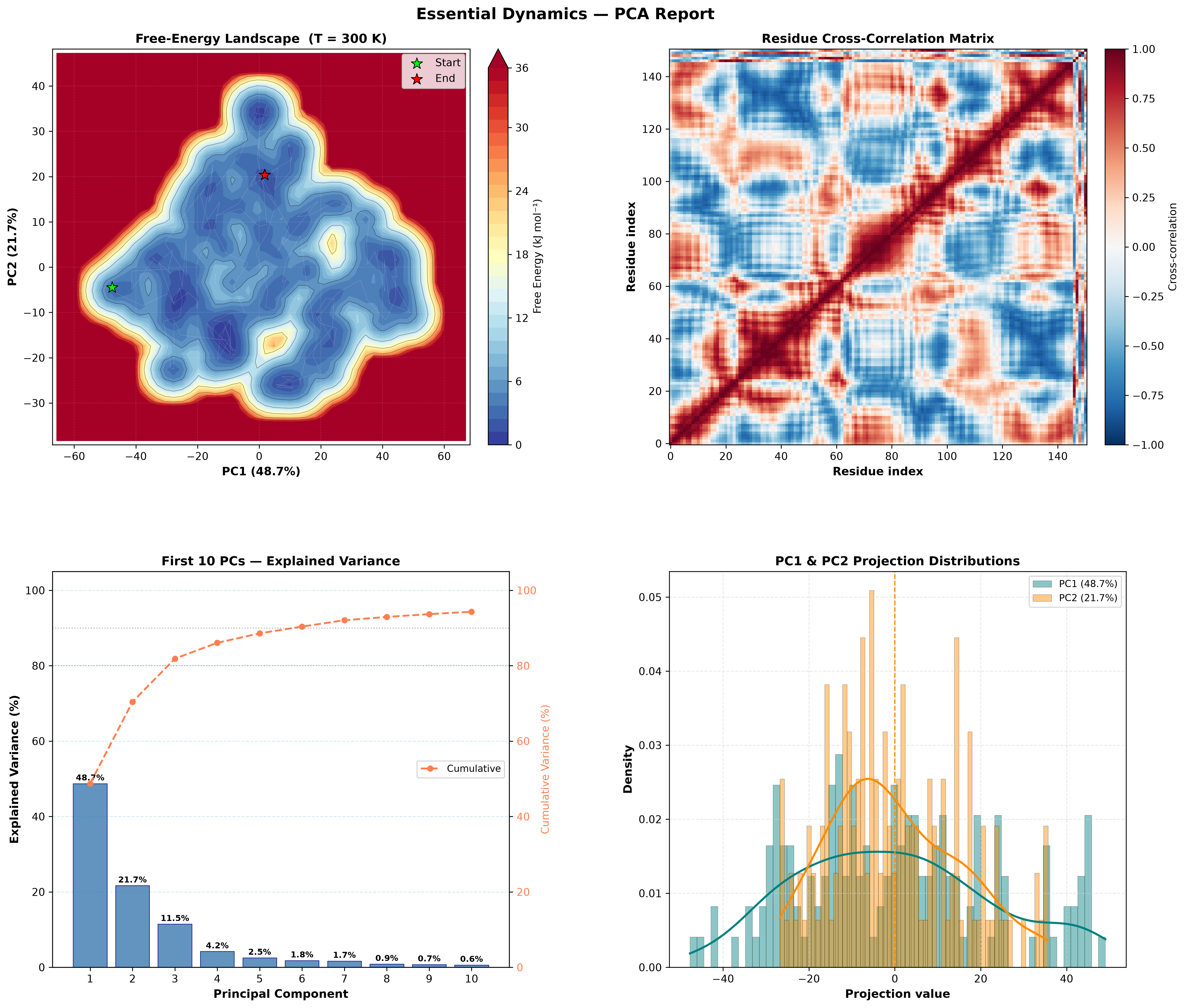
QuickPCA turns long molecular-dynamics trajectories into a single, publication-ready Essential Dynamics report. It loads your trajectory, performs Principal Component Analysis, and renders a four-panel figure with the free-energy landscape, the residue cross-correlation map, the explained-variance profile, and the PC1/PC2 projection distributions — from one command, with no GUI required.
It began life as a drag-and-drop PyMOL script and is now a modern, headless, pip-installable Python package with pluggable NumPy and JAX compute backends.
Why PCA for MD?
Molecular dynamics trajectories carry a massive amount of data. If your protein has 1,000 atoms, each frame has 3,000 coordinates (X, Y, Z). With 10,000 frames that is 30 million data points. PCA analyzes this dataset and reduces its dimensionality: it figures out which atomic movements are just random “noise” and which are the “signals” capturing functionally relevant motions. The algorithm compresses thousands of dimensions down to just a few (PC1, PC2, …) while preserving the most important information.
Unlike common PCA approaches, which construct and diagonalize the covariance matrix, QuickPCA
performs an SVD decomposition directly on the (n_frames × 3N) data matrix. This avoids
the costly step of diagonalizing the covariance matrix, making the approach faster and more
numerically stable, while producing identical principal components. The residue
cross-correlation matrix is subsequently recovered analytically from the PCA eigenvectors and
eigenvalues, without revisiting the raw trajectory data.
Features
- Headless and pip-installable — runs on a laptop, a cluster node, or in CI; no GUI, no display required.
- Pluggable compute backends — a pure NumPy backend out of the box, plus an optional JAX backend for GPU/TPU acceleration.
- Robust trajectory loading — an MDAnalysis-based loader supporting
.nc,.xtc,.trr,.dcdand.pdbformats. - Free-Energy Landscape — Boltzmann-inverted 2-D FEL over PC1/PC2 with Gaussian smoothing.
- Residue cross-correlation — recovered analytically from the PCA eigenbasis.
- Publication-ready reports — a 2×2 matplotlib figure rendered to PNG at 300 dpi.
- Extensible subcommand suite — RMSF, clustering, convergence and interactive report subcommands plug in via an auto-discovered command registry.
- PyMOL plugin — the original drag-and-drop workflow is preserved for interactive use.
Installation
pip install quickpca
QuickPCA targets Python 3.10+ and is installable from PyPI once published.
Optional extras let you pull in only what you need:
pip install "quickpca[jax]"   # GPU/TPU acceleration via JAX
pip install "quickpca[viz]"   # interactive Plotly figures
pip install "quickpca[web]"   # Streamlit web front-end
pip install "quickpca[all]"   # everything above
For development:
pip install -e ".[dev]" # pytest, ruff, mypy, pre-commit
Quickstart
Command line
Run the full load → PCA → FEL → report pipeline in one shot:
quickpca run data/reference.pdb data/trajectory.nc --interval 5
This writes PCA_Report.png to the current directory. Useful options:
quickpca run data/reference.pdb data/trajectory.nc \
    --selection "name CA" \   # MDAnalysis atom selection
    --interval 5 \            # frame stride
    --ncomp 10 \              # principal components to keep
    --temp 300 \              # temperature (K) for the FEL
    --backend numpy \         # compute backend (numpy | jax)
    --output report.png       # output PNG path
List the compute backends available in your environment:
quickpca backends
Python API
from quickpca import compute_pca_from_files, compute_fel, plot_report

# Load a trajectory and run the full PCA pipeline.
pca = compute_pca_from_files(
    "data/reference.pdb",
    "data/trajectory.nc",
    selection="name CA",
    interval=5,
    n_components=10,
    backend="numpy",
)

# Boltzmann-inverted free-energy landscape over PC1/PC2.
fel = compute_fel(pca.projections, temperature=300.0)

# Render the four-panel report to a PNG.
path = plot_report(pca, fel, output="PCA_Report.png")
print(f"Report saved to {path}")

# Inspect the decomposition.
print(f"Backend: {pca.backend}")
print(f"PC1 explains {pca.explained_variance_ratio[0] * 100:.1f}% of variance")
JAX / GPU acceleration
QuickPCA’s compute is isolated behind a small backend interface. The pure-NumPy backend is
always available; installing the JAX extra registers a drop-in jax backend that runs the
alignment and SVD on a GPU or TPU when one is present.
pip install "quickpca[jax]"
quickpca run data/reference.pdb data/trajectory.nc --backend jax
from quickpca import available_backends, compute_pca_from_files

print(available_backends())                       # e.g. ['jax', 'numpy']
pca = compute_pca_from_files(
    "data/reference.pdb", "data/trajectory.nc", backend="jax",
)
Both backends produce identical principal components; the JAX path simply accelerates the heavy linear algebra on accelerators.
Subcommand suite
Beyond run, QuickPCA ships a registry of focused subcommands that are auto-discovered at
startup. Run quickpca --help to see everything available in your install.
| Subcommand | Description |
|---|---|
run |
Full pipeline: load → PCA → FEL → 2×2 report PNG. |
backends |
List the registered compute backends. |
rmsf |
Per-residue root-mean-square fluctuation profile. |
cluster |
Conformational clustering in PC space. |
convergence |
Sampling-convergence diagnostics over the trajectory. |
interactive |
Interactive (HTML/Plotly) report for exploration. |
Some subcommands require optional extras (for example
quickpca[viz]for interactive reports). Subcommands that are not installed simply do not appear in--help.
PyMOL plugin
The classic drag-and-drop workflow still works for interactive sessions:
- Place
quickPCA.pyin the same directory as your PDB and trajectory files. - Open your structure in PyMOL.
- Drag and drop
quickPCA.pyinto the PyMOL window.
Supported trajectory formats: .xtc, .trr, .dcd, .nc.
Example report
QuickPCA produces a single 300-dpi figure with four panels:
- Top-left — Free-Energy Landscape (PC1 vs PC2)
- Top-right — Residue cross-correlation matrix
- Bottom-left — Explained-variance bar chart (with cumulative overlay)
- Bottom-right — PC1 & PC2 projection distributions
Documentation
Full documentation — API reference, backend guide and subcommand details — is published with MkDocs at https://5x5x5x5.github.io/quickpca/.
Citation
If QuickPCA contributes to results presented in a publication, thesis, report, or any other
form of scholarly or professional work, please cite it. Citation metadata is provided in
CITATION.cff; GitHub renders a ready-to-use citation from the
“Cite this repository” button on the repository sidebar.
License
Released under the MIT License.
Author
QuickPCA was developed by Gleb Novikov — The Visual Hub.